43 how to add chart labels in excel

support.microsoft.com › en-us › officeAdd or remove data labels in a chart - support.microsoft.com Depending on what you want to highlight on a chart, you can add labels to one series, all the series (the whole chart), or one data point. Add data labels. You can add data labels to show the data point values from the Excel sheet in the chart. This step applies to Word for Mac only: On the View menu, click Print Layout. How To Add Data Labels In Excel -* Petitmarche Now we need to add the flavor names to the label.now right click on the label and click format data labels. To add or move data labels in a chart, you can do as below steps: Source: . Data labels are used to display source data in a chart directly. Change position of data labels. Source: . The column chart will appear.

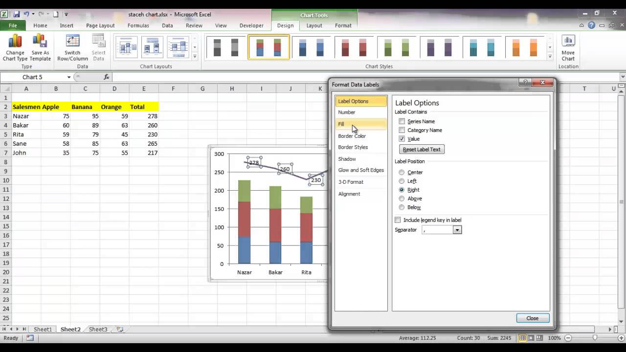
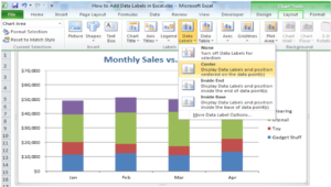
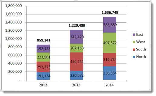
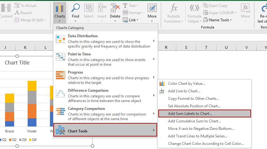
› excel › how-to-add-total-dataHow to Add Total Data Labels to the Excel Stacked Bar Chart Apr 03, 2013 · For stacked bar charts, Excel 2010 allows you to add data labels only to the individual components of the stacked bar chart. The basic chart function does not allow you to add a total data label that accounts for the sum of the individual components. Fortunately, creating these labels manually is a fairly simply process.

How to add chart labels in excel

How to Select Data for Graphs in Excel - Sheetaki Select the blank graph and navigate to the Chart Design tab. Click on the Select Data option. In the Select Data Source dialog box, select the Chart data range text box and type in your range. You may also use your cursor to select the range much faster. Click on the OK button to apply the new data source to your graph. How to Add Axis Labels in Microsoft Excel - Appuals.com Click anywhere on the chart you want to add axis labels to. Click on the Chart Elements button (represented by a green + sign) next to the upper-right corner of the selected chart. Enable Axis Titles by checking the checkbox located directly beside the Axis Titles option. Once you do so, Excel will add labels for the primary horizontal and ... How to Create a Mekko Chart (Marimekko) in Excel - Quick Guide Select the Label Marker series, right-click and choose 'Change Series Chart Type…' The 'Change Chart Type' dialog box will appear. From the series names, select the Label Marker and change the chart type to 'Line with Markers'. #10: Add and Format labels First, select the "Label Marker" series.

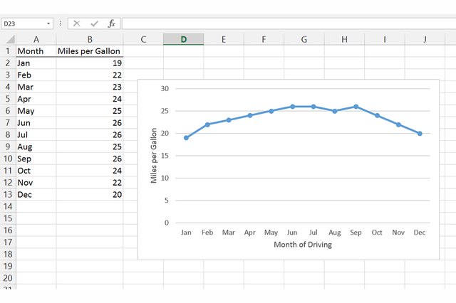
How to add chart labels in excel. peltiertech.com › add-horizontal-line-to-excel-chartAdd a Horizontal Line to an Excel Chart - Peltier Tech Sep 11, 2018 · Let’s focus on a column chart (the line chart works identically), and use category labels of 1 through 5 instead of A through E. Excel doesn’t recognize these categories as numerical values, but we can think of them as labeling the categories with numbers. How to add label to axis in excel chart on mac - WPS Office How to add label to axis in excel online, 2016 and 2019 1. After choosing your chart, go to the Chart Design tab that appears. Axis Titles will appear when you choose them with the drop-down arrow next to Add Chart Element. Choose Primary Horizontal, Primary Vertical, or both from the pop-out menu. 2. How to Print Labels from Excel - Lifewire Choose Start Mail Merge > Labels . Choose the brand in the Label Vendors box and then choose the product number, which is listed on the label package. You can also select New Label if you want to enter custom label dimensions. Click OK when you are ready to proceed. Connect the Worksheet to the Labels How to Add Axis Titles in a Microsoft Excel Chart - How-To Geek Select your chart and then head to the Chart Design tab that displays. Click the Add Chart Element drop-down arrow and move your cursor to Axis Titles. In the pop-out menu, select "Primary Horizontal," "Primary Vertical," or both. If you're using Excel on Windows, you can also use the Chart Elements icon on the right of the chart.

How to add data labels in excel to graph or chart (Step-by-Step) 1. Select a data series or a graph. After picking the series, click the data point you want to label. 2. Click Add Chart Element Chart Elements button > Data Labels in the upper right corner, close to the chart. 3. Click the arrow and select an option to modify the location. 4. How To Add a Legend to a Chart in Excel (2 Methods, FAQs) Another way is to select the "Chart Design" tab in the command ribbon, navigate to "Legend" through the "Add Chart Element" menu and select "None." Additionally, you can right-click on the existing legend and select "Delete" to remove it. Can you change the information in the legend? How to Add Leader Lines in Excel? - GeeksforGeeks Step 1: Select a range of cells for which you want to make a line chart. Step 2: Go to Insert Tab and select Recommended Charts. A dialogue box name Insert Chart appears. Step 3: Click on All Charts and select Line. Click Ok. Step 4: A line chart is embedded in the worksheet. Step 5: Go to Chart Design Tab and select Add Chart Element . Adding Data Labels to Your Chart (Microsoft Excel) - ExcelTips (ribbon) To add data labels in Excel 2013 or later versions, follow these steps: Activate the chart by clicking on it, if necessary. Make sure the Design tab of the ribbon is displayed. (This will appear when the chart is selected.) Click the Add Chart Element drop-down list. Select the Data Labels tool.

Label line chart series - Get Digital Help To label each line we need a cell range with the same size as the chart source data. Simply copy the chart source data range and paste it to your worksheet, then delete all data. All cells are now empty. Copy categories (Regions in this example) and paste to the last column (2018). Those correspond to the last data points in each series. How to☝️Create a Pie of Pie Chart in Excel - SpreadsheetDaddy Select the Add Data Labels option. If you want the labels to be more visually appealing, you can change their color as well. Select the labels. Go to the Home menu. Navigate to the Font section and click on the Font Color option. Choose a color that works best for your chart. How to Create and Customize a Treemap Chart in Microsoft Excel Either right-click the chart and pick "Format Chart Area" or double-click the chart to open the sidebar. On Windows, you'll see two handy buttons on the right of your chart when you select it. With these, you can add, remove, and reposition Chart Elements. And you can pick a style or color scheme with the Chart Styles button. Custom Chart Data Labels In Excel With Formulas - How To Excel At Excel Select the chart label you want to change. In the formula-bar hit = (equals), select the cell reference containing your chart label's data. In this case, the first label is in cell E2. Finally, repeat for all your chart laebls. If you are looking for a way to add custom data labels on your Excel chart, then this blog post is perfect for you.

Create Custom Data Labels in Excel Charts - YouTube

› solutions › excel-chatHow to Insert Axis Labels In An Excel Chart | Excelchat Figure 1 – How to add axis titles in Excel. Add label to the axis in Excel 2016/2013/2010/2007. We can easily add axis labels to the vertical or horizontal area in our chart. The method below works in the same way in all versions of Excel. How to add horizontal axis labels in Excel 2016/2013 . We have a sample chart as shown below; Figure 2 ...

How to Add an Axis Title to an Excel Chart | Techwalla

How to make a quadrant chart using Excel | Basic Excel Tutorial To create it, follow these steps 1. Click on an empty cell 2. Go to the Insert tab 3. On the Charts dialog box, select the X Y (Scatter) to display all types of charts. 5. Click Scatter. An empty chart will appear on your worksheet. Add values to the chart. 1. Right-click on the empty chart area and choose 'Select Data.' 2.

30 How To Add Label To Excel Chart - Labels Database 2020

How to Add Total Values to Stacked Bar Chart in Excel Step 4: Add Total Values. Next, right click on the yellow line and click Add Data Labels. Next, double click on any of the labels. In the new panel that appears, check the button next to Above for the Label Position: Next, double click on the yellow line in the chart. In the new panel that appears, check the button next to No line:

Excel Course: Inserting Graphs

How to Add Two Data Labels in Excel Chart (with Easy Steps) Table of Contents hide. Download Practice Workbook. 4 Quick Steps to Add Two Data Labels in Excel Chart. Step 1: Create a Chart to Represent Data. Step 2: Add 1st Data Label in Excel Chart. Step 3: Apply 2nd Data Label in Excel Chart. Step 4: Format Data Labels to Show Two Data Labels. Things to Remember.

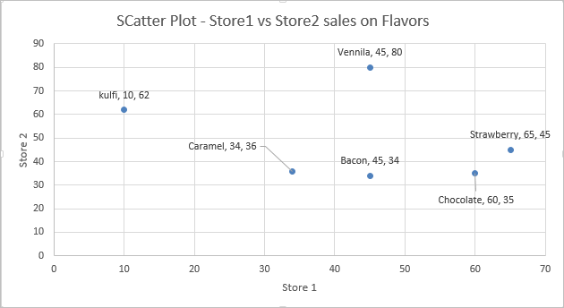
Add Custom Labels to x-y Scatter plot in Excel - DataScience Made Simple

Chart.ApplyDataLabels method (Excel) | Microsoft Docs Syntax expression. ApplyDataLabels ( Type, LegendKey, AutoText, HasLeaderLines, ShowSeriesName, ShowCategoryName, ShowValue, ShowPercentage, ShowBubbleSize, Separator) expression A variable that represents a Chart object. Parameters Example This example applies category labels to series one on Chart1. VB Copy Charts ("Chart1").SeriesCollection (1).

Add Total Label On Stacked Bar Chart In Excel - YouTube

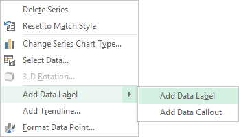
› documents › excelHow to add data labels from different column in an Excel chart? This method will introduce a solution to add all data labels from a different column in an Excel chart at the same time. Please do as follows: 1. Right click the data series in the chart, and select Add Data Labels > Add Data Labels from the context menu to add data labels. 2.

Improve your X Y Scatter Chart with custom data labels

spreadsheeto.com › axis-labelsHow to Add Axis Labels in Excel Charts - Step-by-Step (2022) How to Add Axis Labels in Excel Charts – Step-by-Step (2022) An axis label briefly explains the meaning of the chart axis. It’s basically a title for the axis. Like most things in Excel, it’s super easy to add axis labels, when you know how. So, let me show you 💡. If you want to tag along, download my sample data workbook here.

Creating a chart with dynamic labels - Microsoft Excel 2013

How to Show Percentages in Stacked Column Chart in Excel? Follow the below steps to show percentages in stacked column chart In Excel: Step 1: Open excel and create a data table as below. Step 2: Select the entire data table. Step 3: To create a column chart in excel for your data table. Go to "Insert" >> "Column or Bar Chart" >> Select Stacked Column Chart. Step 4: Add Data labels to the chart.

Creating Pie Chart and Adding/Formatting Data Labels (Excel) - YouTube

Make better Excel Charts by adding graphics or pictures There's two ways to add images or graphics to an Excel chart. In this article we'll show how to overlay graphics over charts like the Pie Chart. In Better looking Excel Charts we'll show how to replace a colored chart block with an image. Insert picture into a chart . We have a basic 2D pie chart like this, very boring, very dull.

How to Add Data Labels in Excel - Excelchat | Excelchat

How to format axis labels individually in Excel - SpreadsheetWeb How to add custom formatting to a chart's axis. Double-click on the axis you want to format. Double-clicking opens the right panel where you can format your axis. Open the Axis Options section if it isn't active. You can find the number formatting selection under Number section. Select Custom item in the Category list.

34 How To Label A Chart In Excel - Label Ideas 2020

How to Add a Vertical Line to Charts in Excel - Statology This tutorial provides a step-by-step example of how to add a vertical line to the following line chart in Excel: Let's jump in! Step 1: Enter the Data. Suppose we would like to create a line chart using the following dataset in Excel: Step 2: Add Data for Vertical Line. Now suppose we would like to add a vertical line located at x = 6 on the ...

How to Show Percentages in Stacked Bar and Column Charts in Excel

How to Make a Pie Chart in Excel & Add Rich Data Labels to The Chart! 2) Go to Insert> Charts> click on the drop-down arrow next to Pie Chart and under 2-D Pie, select the Pie Chart, shown below. 3) Chang the chart title to Breakdown of Errors Made During the Match, by clicking on it and typing the new title.

How-to Add Custom Labels that Dynamically Change in Excel Charts - Excel Dashboard Templates

How To Create Labels In Excel - BT123 - booktable.info How to Print Labels from Excel from . The "label options" window will appear. Choose supplier of label sheets under label information. How to add brackets to the existing code. Source: . Click "labels" on the left side to make the "envelopes and labels" menu appear. In our case, it's c3. Source: www ...

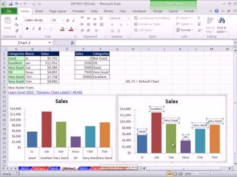
Excel Magic Trick 804: Chart Double Horizontal Axis Labels & VLOOKUP to Assign Sales Category ...

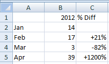
chandoo.org › wp › change-data-labels-in-chartsHow to Change Excel Chart Data Labels to Custom Values? May 05, 2010 · We all know that Chart Data Labels help us highlight important data points. When you “add data labels” to a chart series, excel can show either “category” , “series” or “data point values” as data labels. But what if you want to have a data label that is altogether different, like this:

How to add total labels to stacked column chart in Excel?

All About Chart Elements in Excel - Add, Delete, Change - Excel Unlocked The fourth option from the chart element item is for the chart title. On clicking the right arrow, we will find there are three options to change the position of the chart to keep it either above the chart or to overlap it on the chart. More options open the format chart title pane on the left. By default, Excel writes the text string "Chart ...

34 How To Add Label To Excel Chart

How to add text labels on Excel scatter chart axis Stepps to add text labels on Excel scatter chart axis 1. Firstly it is not straightforward. Excel scatter chart does not group data by text. Create a numerical representation for each category like this. By visualizing both numerical columns, it works as suspected. The scatter chart groups data points. 2. Secondly, create two additional columns.

Show Trend Arrows in Excel Chart Data Labels

Adding Data Labels to the Inside Ring of a Sunburst Chart : r/excel Follow the submission rules -- particularly 1 and 2. To fix the body, click edit. To fix your title, delete and re-post. Include your Excel version and all other relevant information Failing to follow these steps may result in your post being removed without warning. I am a bot, and this action was performed automatically.

Automatically update data labels on Excel chart (Excel 2016) - Stack Overflow

How to Create a Mekko Chart (Marimekko) in Excel - Quick Guide Select the Label Marker series, right-click and choose 'Change Series Chart Type…' The 'Change Chart Type' dialog box will appear. From the series names, select the Label Marker and change the chart type to 'Line with Markers'. #10: Add and Format labels First, select the "Label Marker" series.

Share :