42 add data labels to waterfall chart

Excel Waterfall Charts • My Online Training Hub For Excel 2007 or 2010 users there is no easy way to add labels. Adding labels to the chart will result in a mess which you have to tidy up. To tidy them up select each label box with 2 single left-clicks, then click in the formula bar and type = then click on the cell containing the label value in the chart source data table and press ENTER. Not able to add data label in waterfall chart using ggplot2 I am trying to plot waterfall chart using ggplot2. When I am placing the data labels it is not putting in the right place. Below is the code I am using dataset <- data.frame(TotalHeadcount =...

Add data labels, notes, or error bars to a chart - Google You can add data labels to a bar, column, scatter, area, line, waterfall, histograms, or pie chart. Learn more about chart types. On your computer, open a spreadsheet in Google Sheets. Double-click the chart you want to change. At the right, click Customize Series. Check the box next to “Data labels.”

Add data labels to waterfall chart

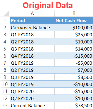
How to add Data Label to Waterfall chart - excelforum.com Add data labels to this added series, position the labels above the points. Here are options for what's in the labels: 1. Manually edit the text of the labels. 2. Select each label (two single clicks, one selects the series of labels, the second selects the individual label). Don't click so much as the cursor starts blinking in the label. How to Create and Customize a Waterfall Chart in Microsoft Excel Start by selecting your data. You can see below that our data begins with a starting balance, includes incoming and outgoing funds, and wraps up with an ending balance. You should arrange your data similarly. Go to the Insert tab and the Charts section of the ribbon. Click the Waterfall drop-down arrow and pick "Waterfall" as the chart type. Introducing the Waterfall chart—a deep dive to a more streamlined chart ... To start, select your data and then under the Insert tab click the Recommended Charts button. The list of recommended charts is displayed. Select the Waterfall recommendation to preview the chart with your selected data. The All Charts tab allows direct insertion of Waterfall charts. You can also use the ribbon to insert the Waterfall chart ...

Add data labels to waterfall chart. How to add data labels from different column in an Excel chart? This method will guide you to manually add a data label from a cell of different column at a time in an Excel chart. 1. Right click the data series in the chart, and select Add Data Labels > Add Data Labels from the context menu to add data labels. 2. Click any data label to select all data labels, and then click the specified data label to ... How to create a waterfall chart in Google Sheets Create a new data table for the waterfall chart. Directly adjacent to the original data, make a copy of the row labels, then add four new columns: Base; Endpoints; Positive; Negative, as shown below: Step 3: Formulas for our waterfall chart. Add the following formulas to the table (click to enlarge): Waterfall Charts in Excel - A Beginner's Guide | GoSkills Go to the Insert tab, and from the Charts command group, click the Waterfall chart dropdown. The icon looks like a modified column chart with columns going above and below the horizontal axis. Click Waterfall (the first chart in that group). Excel will insert the chart on the spreadsheet which contains your source data. How to Create a Waterfall Chart in Excel and PowerPoint - Smartsheet You're almost finished. You just need to change the chart title and add data labels. Click the title, highlight the current content, and type in the desired title. To add labels, click on one of the columns, right-click, and select Add Data Labels from the list. Repeat this process for the other series.

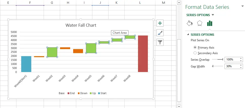
How to Set the Total Bar in an Excel Waterfall Chart Format Data Point Option. To set a total from the formatting pane, you need to either right-click and navigate to Format Data Point…, or first click on the data point you want to isolate, and navigate to Format>Format Pane>Format Data Point. Either way, it's much quicker to simply right-click to set as total, as shown on the left. Create a waterfall chart - support.microsoft.com Connector lines connect the end of each column to the beginning of the next column, helping show the flow of the data in the chart. To hide the connector lines, right-click a data series to open the Format Data Series task pane, and uncheck the Show connector lines box. To show the lines again, check the Show connector lines box. Add Data Points to Existing Chart – Excel & Google Sheets Adding Single Data point. Add Single Data Point you would like to ad; Right click on Line; Click Select Data . 4. Select Add . 5. Update Series Name with New Series Header. 6. Update Values . Final Graph with Single Data point . Add a Single Data Point in Graph in Google Sheets Add a Horizontal Line to an Excel Chart - Peltier Tech 11.09.2018 · Since they are independent of the chart’s data, they may not move when the data changes. And sometimes they just seem to move whenever they feel like it. The examples below show how to make combination charts, where an XY-Scatter-type series is added as a horizontal line to another type of chart. Add a Horizontal Line to an XY Scatter Chart

Excel 2016 Waterfall Chart - How to use, advantages and ... - Xelplus To use the new Excel 2016 Waterfall Chart, highlight the data area including the empty cell right above the categories and Insert > Waterfall Chart. It will give you three series: Increase, Decrease and Total. At this point you will see the first two, but not the Total. How to Create a Waterfall Chart in Excel - Automate Excel Right-click on any column and select "Add Data Labels." Immediately, the default data labels tied to the helper values will be added to the chart: But that is not exactly what we are looking for. To work around the issue, manually replace the default labels with the custom values you prepared beforehand. Double-click the data label you want ... How to Create a Waterfall Chart Template | GoCardless Select the data you want to highlight, including row and column headers. Go to the 'Insert' tab, click on 'Column Charts', and then select the 'Stacked Chart' option. Step 3: Convert the stacked chart to a waterfall chart Now you can convert the stacked chart to a waterfall chart format. To do this, you'll need to hide the 'Base' series from view. Data labels position in Waterfall chart - GrapeCity Discussion of topic Data labels position in Waterfall chart in General Discussion forum. Discussion of topic Data labels position in Waterfall chart in General Discussion forum. ... You may achieve the desired behavior by handling the rendered event of DataLabel and adding a new label to the desired position. Please refer to the sample below ...

VBA macro: change font of series 1 data labels of waterfall chart : excel

Waterfall Chart: Excel Template & How-to Tips | TeamGantt To add a title to your chart: Click on your chart and look for "chart options" in the formatting palette. Click on the chart title box to name your chart. If you want to add a data label to show specific numbers for each column, you can do that. Right click on one of your columns and select "Add Data Labels" from the dropdown.

Waterfall chart using totals from multiple sheets (or data sources)

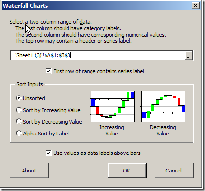
How to create waterfall chart in Excel 2016, 2013, 2010 25.07.2014 · You can choose to make either a standard Waterfall Chart or a Stacked Waterfall Chart. It is not necessary to enter any formulas, just select your data, click the Waterfall Chart command in the Ribbon, set a few options, click OK and Excel bridge graph is ready. In addition to custom charts, the add-in provides you with different Chart, Data and General Tools to make …

Navigating Waterfall Charts for Page Load and Transaction Tests - ThousandEyes Documentation

Formatting of data labels for waterfall charts in shared Powerpoint ... Formatting of data labels for waterfall charts in shared Powerpoint (365) file is not shown consistently with different people who have access I have a presentation that contains a waterfall chart that was created in Powerpoint. Data labels are added to the chart and numbers are shown without decimals but with thousand separator.

How to Create a Waterfall Chart in Excel and PowerPoint

4 steps: How to Create Waterfall Charts in Excel 2013 Add data labels by right-clicking one of the series and selecting "Add data labels…" Add labels to each of the series apart from the invisible column. Select the data labels and make them bold, change colour as appropriate. The finished chart should look something similar to the one below. Download the completed version here. grab user attention

How to Make a Simple Waterfall Chart - The Data School Australia

Create waterfall or bridge chart in Excel - ExtendOffice At last, give a name for the chart, and now, you will get the waterfall chart successfully, see screenshot: Note: Sometimes, you may want to add data labels to the columns. Please do as follows: 1. Select the series that you want to add the label, then right click and choose the Add Data Labels option, see screenshot: 2.

Creating a waterfall chart in TIBCO Spotfire | TIBCO Community

Excel Waterfall Chart: How to Create One That Doesn't Suck - Zebra BI Ideally, you would create a waterfall chart the same way as any other Excel chart: (1) click inside the data table, (2) click in the ribbon on the chart you want to insert. ... in Excel 2016 Microsoft decided to listen to user feedback and introduced 6 highly requested charts in Excel 2016, including a built-in Excel waterfall chart.

Waterfall Chart in Excel - DataScience Made Simple

How to Use Cell Values for Excel Chart Labels - How-To Geek 12.03.2020 · Make your chart labels in Microsoft Excel dynamic by linking them to cell values. When the data changes, the chart labels automatically update. In this article, we explore how to make both your chart title and the chart data labels dynamic. We have the sample data below with product sales and the difference in last month’s sales.

Waterfall Chart - Page 2 of 2 - Beat Excel!

Waterfall charts - Google Docs Editors Help Customize a waterfall chart. On your computer, open a spreadsheet in Google Sheets. Double-click the chart you want to change. At the right, click Customize. Chart style: Change how the chart looks, or add and edit connector lines. Chart & axis titles: Edit or format title text. Series: Change column colors, add and edit subtotals and data labels.

Waterfall Add-in — The Spreadsheet Guru

Add Totals to Stacked Bar Chart - Peltier Tech 15.10.2019 · In Label Totals on Stacked Column Charts I showed how to add data labels with totals to a stacked vertical column chart. That technique was pretty easy, but using a horizontal bar chart makes it a bit more complicated. In Add Totals to Stacked Column Chart I discussed the problem further, and provided an Excel add-in that will apply totals labels to stacked column, …

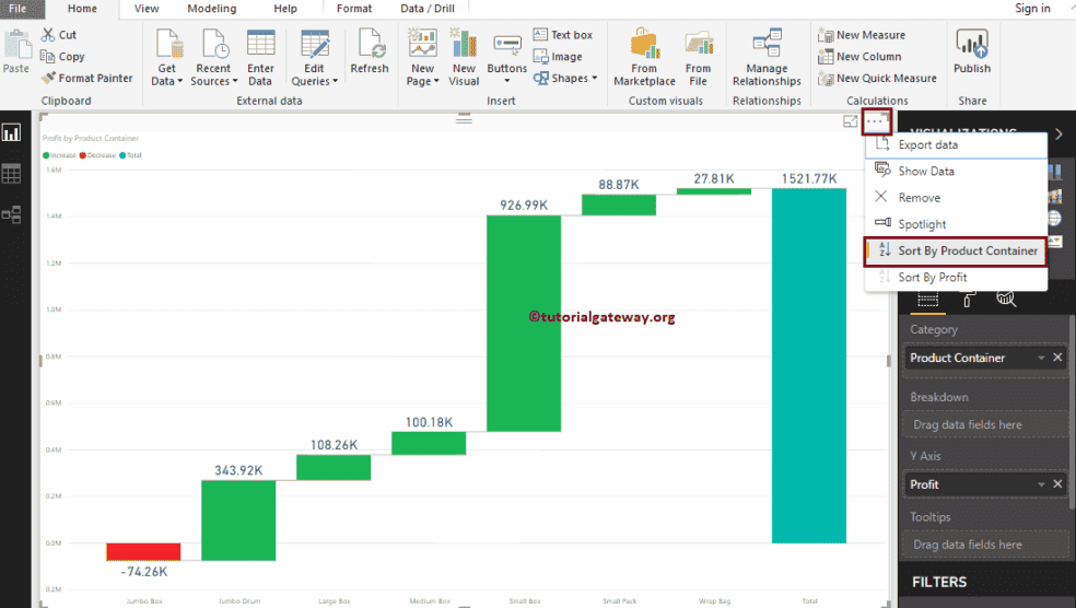
Waterfall Chart in Power BI

Waterfall Chart in Excel (Examples) | How to Create Waterfall Chart? Select the blue bricks and right-click and select the option "Add Data Labels". Then you will get the values on the bricks; for better visibility, change the brick color to light blue. Double click on the "chart title" and change to the waterfall chart. If you observe, we can see both monthly sales and accumulated sales in the singles chart.

Best 171 DataViz - Components images on Pinterest | Other

Create Excel Waterfall Chart Template - Download Free Template Jun 09, 2022 · Right-click on the waterfall chart and go to Select Data. Add a new series using cell I4 as the series name, I5 to I11 as the series values, and C5 to C11 as the horizontal axis labels. Right-click on the waterfall chart and select Change Chart Type. Change the chart type of the data label position series to Scatter. Make sure the Secondary ...

PowerPointing – How to Create a Waterfall Chart in PowerPoint

How to add Data markers in Waterfall chart in Plotly I am trying to plot waterfall chart with the following code. The only issue I am facing currently is the data marker which is not at the correct place. I want the data marker to be just below the end of each bar. Attached the screenshot of the waterfall chart. So for the first bar, I need the data marker to be just below the end of red bar.

How to Create a Waterfall Chart in Excel - Automate Excel

Add or remove data labels in a chart - support.microsoft.com Click the data series or chart. To label one data point, after clicking the series, click that data point. In the upper right corner, next to the chart, click Add Chart Element > Data Labels. To change the location, click the arrow, and choose an option. If you want to show your data label inside a text bubble shape, click Data Callout.

What Is a Waterfall Chart and Why Would I Need One – Contextures Blog

Create Waterfall Chart, Auto update Bar Colour and Data labels ... Learn to create linked / automated Waterfall chart with distinct colours for up and down variances, data labels update automatically, graph colour changes au...

Waterfall Chart Templates (Excel 2010 and 2013) – Edward Bodmer – Project and Corporate Finance

How To Make Waterfall Charts in Google Sheets - UbuntuPIT Get Your Waterfall Charts Prepared In this step, first, select the entire datasheet and click on the Insert option from the above menu. By doing so, you'll get an option called Chart in the submenu. Now, click on it. Once you've completed the above instruction correctly, a waterfall chart will appear on your Google sheets like the below one.

Top N, Annotations, Stacking & Latest Features - Waterfall Power BI Visual

Add & edit a chart or graph - Computer - Google Docs Editors Help The legend describes the data in the chart. Before you edit: You can add a legend to line, area, column, bar, scatter, pie, waterfall, histogram, or radar charts.. On your computer, open a spreadsheet in Google Sheets.; Double-click the chart you want to change. At the right, click Customize Legend.; To customize your legend, you can change the position, font, style, and color.

How to create a Waterfall Chart in Excel

Introducing the Waterfall chart—a deep dive to a more streamlined chart ... To start, select your data and then under the Insert tab click the Recommended Charts button. The list of recommended charts is displayed. Select the Waterfall recommendation to preview the chart with your selected data. The All Charts tab allows direct insertion of Waterfall charts. You can also use the ribbon to insert the Waterfall chart ...

Share :